3.13. Rule-based Modeling with BioNetGen, BNGL, and RuleBender
3.13.1. Description of Rule-based Modeling, BioNetGen, BNGL, and RuleBender
As the Summary of the The BioNetGen Online Manual 1 says:
Rule-based modeling involves the representation of molecules as structured objects and molecular interactions as rules for transforming the attributes of these objects. The approach is notable in that it allows one to systematically incorporate site-specific details about protein-protein interactions into a model for the dynamics of a signal-transduction system, but the method has other applications as well, such as following the fates of individual carbon atoms in metabolic reactions. The consequences of protein-protein interactions are difficult to specify and track with a conventional modeling approach because of the large number of protein phosphoforms and protein complexes that these interactions potentially generate.
- 1
Contributors: James R. Faeder, Michael L. Blinov, William S. Hlavacek, Leonard A. Harris, Justin S. Hogg, Arshi Arora
3.13.2. BNGL and RuleBender Basic Functionality
This section demonstrates the basic functionality of the BioNetGen language (BNGL) and RuleBender, which is the BioNetGen IDE.
Obtain BioNetGen, RuleBender, and NFsim by following the directions at BioNetGen quick start. Java and Perl must be installed. The BioNetGen Quick Reference Guide summarizes much of BioNetGen and its ecosystem in four pages.
Run RuleBender, which can:
Edit and save BNGL models
Create new BNGL models
Run BNGL models in a simulator
Print simulator debugging and logging outputs
Plot species population predictions generated by simulation
Diagram and inspect molecular types and rules
RuleBender comes with many sample models written in BNGL. Open the birth-death model by clicking on File -> New BioNegGen Project -> OK -> Select a Sample -> birth-death -> Type Project Name ‘birth-death_test’.
The birth-death model contains just one specie, A, with no initial population:
begin species
  A() 0
end species
And it contains just two rules:
birth: 0 -> A() kp1
death: A() -> 0 km1
It’s a simple model. Birth creates species A, while death destroys it.
Irreversible rules have the form:
rule_name: reactants -> products forward_rate_law
Reversible rules have the form:
rule_name: reactants <-> products forward_rate_law, reverse_rate_law
The null (0) reactants and products in these rules allow
A to be created from nothing and destroyed without a trace.
These rules aren’t mass balanced, of course, but ignore that for now.
Simulate the model. Both ODE and SSA solvers are run, each for 50 seconds:
saveConcentrations()
simulate({suffix=>"ode",method=>"ode",t_end=>50,n_steps=>500})
resetConcentrations()
simulate({suffix=>"ssa",method=>"ssa",t_end=>50,n_steps=>500})
Before you look at the results, try to answer these questions:
What population do you expect the model will predict for
A?How do you expect the population to vary over the 50 sec for the ODE and SSA models?
Now look at the results by clicking on the birth-death_ode.gdat and birth-death_ssa.gdat and
tabs.
Did you anticipate the model’s predictions?
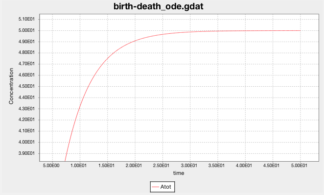
The ODE solver predicts that the population of A grows smoothly and rises asymptotically to 50.
(The y-axis label says ‘Concentration’, but it should say ‘population’.
The model doesn’t have a volume, so it cannot calculate concentration.)
Does this make sense?
The system reaches equilibrium when A is created at the same rate that it is destroyed.
In equilibrium, \(dA(t)/dt = 0\).
The birth rule creates \(A\) at the constant rate of kp1 or 10/sec.
And the death rule destroys the existing \(A\) at a rate of km1 or 0.2 of per second.
In this continuous ODE model, the quantity of \(A\) is then given by
Taking the time derivative and setting it equal to 0, we get
whose solution is \(A = 50\), as predicted by the ODE solver.
Note that ODE integrators approximate species populations (or concentrations)
as non-negative real numbers, whereas populations are really
non-negative integers. You can visualize this
in RuleBender by zooming in on the
birth-death_ode.gdat plot. Select a rectangle of the plot from upper-left to lower-right
to see the smooth, real-valued predictions.
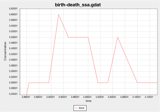
Look at SSA’s predictions for the population of A. What happens when you
greatly increase the simulation’s end time (t_end)?
Zooming in shows that SSA predicts the population as a non-negative integer at each sampled time step.
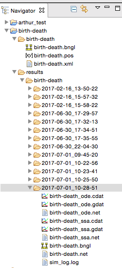
You can find the raw inputs and outputs for each simulation run in the results subdirectory
of the birth-death project.
Raw predictions are in cdat files. Data for the above plot are in birth-death_ssa.cdat:
3.860000000000e+01  5.100000000000e+01
3.880000000000e+01  5.300000000000e+01
3.900000000000e+01  5.300000000000e+01
3.920000000000e+01  5.300000000000e+01
3.940000000000e+01  5.600000000000e+01
3.960000000000e+01  5.500000000000e+01
3.980000000000e+01  5.500000000000e+01
4.000000000000e+01  5.500000000000e+01
4.020000000000e+01  5.300000000000e+01
4.040000000000e+01  5.300000000000e+01
4.060000000000e+01  5.500000000000e+01
4.080000000000e+01  5.400000000000e+01
4.100000000000e+01  5.300000000000e+01
4.120000000000e+01  5.300000000000e+01
4.140000000000e+01  5.300000000000e+01
3.13.3. Exercises
What happens when you change the rate law constants? Adjust them so the equilibrium population is 200. Adjust them so that the model does not reach an equilibrium. Can they be adjusted to reduce the variance of the SSA predictions?
Debugging models is easier when re-executing a simulation run produces identical output, that is, reproduces a previous run. Reproducibility is also an important feature of the scientific method. Can you program RuleBender and BNGL to exactly reproduce these SSA predictions? (I’m not aware of a way to do so.)
3.13.4. Molecular sites, their states, and bonds
In this section we create a new BNGL model. Follow chapter 3 of the
Rule-Based Modeling of
Signal Transduction: A Primer.
Make a new project
by clicking on and typing
File -> New BioNegGen Project -> OK ->
Select a Sample -> template.bngl -> Type Project Name ‘signal_transduction’.
template.bngl provides a template BNGL program with initialized blocks.